From Zero-Shot to Production: A Practical Image Classification Workflow

From Zero-Shot to Production: A Practical Image Classification Workflow

Introduction

This project started with a simple internal question:

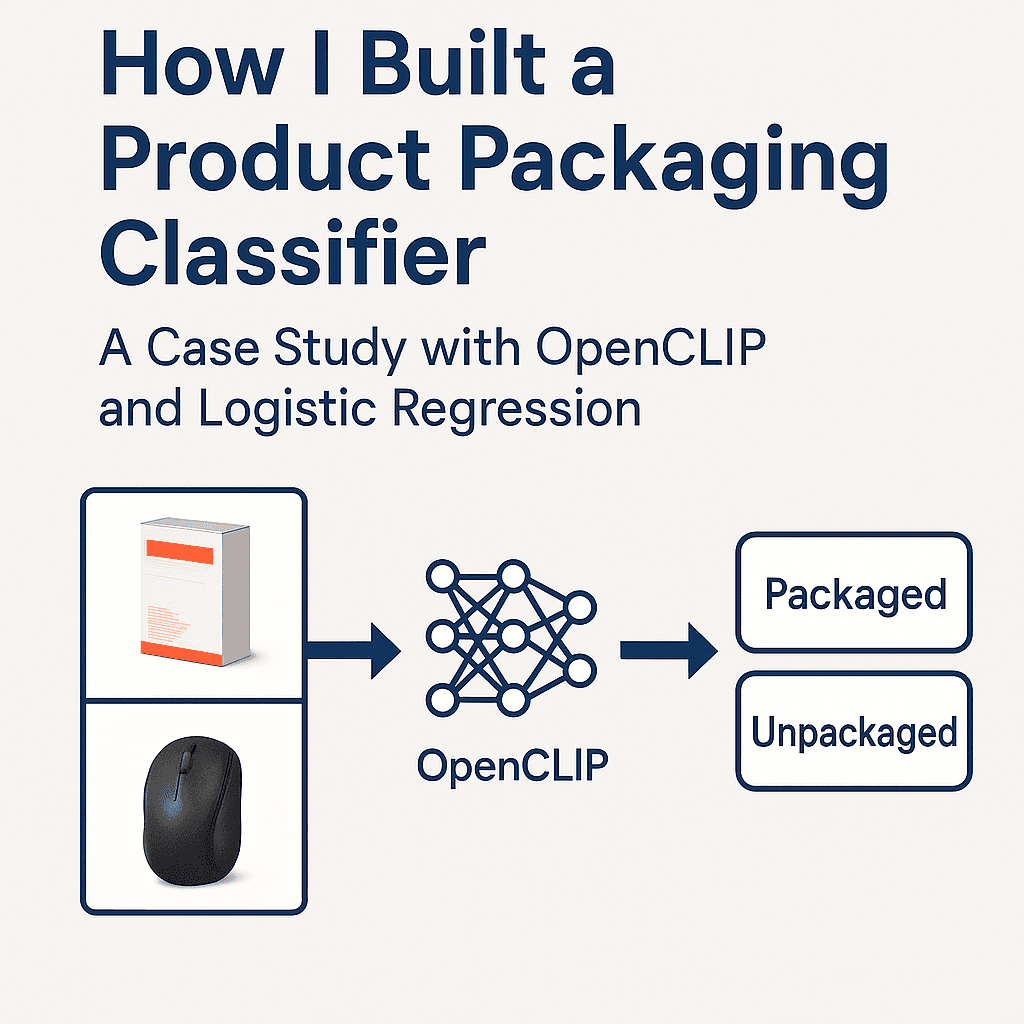
Can we automatically separate packaged vs. unpackaged product images in our catalog?

Vendors often send us ZIP files containing tens of thousands of mixed images - packaged shots, loose items, lifestyle photos, renders, and close-ups. There's no metadata, no naming structure, and no consistency.

Manually sorting 45,000+ images wasn't realistic. Instead of treating this as a full "ML initiative," I approached it the way I've tackled projects in my homelab or at school:

• start simple
• build only what's needed
• iterate as you learn
• keep the system practical

That mindset led to a lightweight ML workflow that handled the entire dataset with only a few hundred human labels.

TL;DR

I built a small internal ML system that uses:

• Zero-shot OpenCLIP embeddings to start with no labels
• A Logistic Regression classifier for fast supervised learning
• Decision fusion: zero-shot + classifier + clustering
• Embedding caching + batch GPU inference for efficiency
• Active learning to reduce labeling effort
• Two lightweight UIs (Qt + Flask) for quick labeling

It was a focused project, but it solved a real internal bottleneck and sharpened my applied ML engineering skills.

System Setup at a Glance

• IMAGE_DIR=all_images, outputs copied to classified/packaged and classified/unpackaged
• Embeddings cached in image_embeds_cache.pkl with model/pretrained stamped to avoid stale reuse
• Labels stored in labeled_images.pkl, classifier in trained_classifier.pkl
• Adaptive batching: defaults to 16 on GPU, 8 on CPU to balance throughput and memory
• Confidence guardrails: CONFIDENCE_MARGIN=1.10, active-learning queue capped at 1,000 per session
• Runs on CUDA if available, otherwise CPU; web UI via Flask, desktop UI via PySide6 Qt

Step 1: Starting With Zero-Shot CLIP

Because we had zero labeled images, I began with OpenCLIP ViT-H-14.

I created simple text prompts to anchor packaged vs. unpackaged semantics:

packaged_prompts = [
    "a product in packaging",
    "a boxed product",
    "retail packaging",
]

unpackaged_prompts = [
    "a product without packaging",
    "product only, no box",
    "item removed from packaging",
]

CLIP converts these into text embeddings:

with torch.no_grad():
    text_tokens = tokenizer(all_prompts).to(device)
    text_features = model.encode_text(text_tokens)
    text_features /= text_features.norm(dim=-1, keepdim=True)

At this stage, zero-shot predictions were rough but surprisingly useful. They formed the starting point for active learning and gave the first signal for classification (the zero-shot step is text–image similarity; the Logistic Regression later uses the image embeddings, not a “zero-shot embedding”).

Implementation notes:

• Model: open_clip.create_model_and_transforms("ViT-H-14", "laion2b_s32b_b79k")
• Tokenization and encoding happen once at startup; embeddings are L2-normalized for clean cosine sims
• Runs in half precision on GPU for speed; AMP autocast mainly benefits GPU paths (it does not speed up CPU)
• CLIP packaging semantics are prompt-sensitive; packaging vs. unpackaged is not a native class, so prompts need tuning and still fluctuate

Source: Pinecone guide to multi-modal ML with CLIP.

Source: LearnOpenCV CLIP tutorial.

Step 2: Adding a Lightweight Supervised Layer

Once I labeled a small set of examples, I trained a Logistic Regression classifier on the CLIP embeddings:

clf = LogisticRegression(max_iter=2000)
clf.fit(X_train, y_train)

This was intentional:

• it trains fast
• it works well on small datasets
• it updates instantly
• no GPU required

It quickly began outperforming zero-shot predictions, even with <200 labeled samples. The probabilities are not calibrated (especially with few labels), so they are best treated as relative scores, not ground-truth confidence.

Persistence and guardrails:

• Labels are saved to labeled_images.pkl; classifier is persisted to trained_classifier.pkl
• Training only kicks in after at least 10 samples with both classes represented
• The Qt and web labelers retrain every 10 labels so the model keeps getting sharper during a session

Source: Wikimedia Commons (“Logistic-curve.svg”).

Step 3: Decision Fusion

Vendor data is extremely inconsistent. Images vary in lighting, angle, background, and composition.

To stabilize predictions, I combined three signals:

1. Zero-shot confidence
2. Classifier probability
3. KMeans cluster prior

The fusion logic looked like this:

if clf is not None:
    prob_packaged = clf.predict_proba(feat.reshape(1, -1))[0, 1]
    return "packaged" if prob_packaged >= 0.5 else "unpackaged"

zs_label, sims = zero_shot_label(feat)
cluster = cluster_labels[idx]

# fallback heuristics
if zs_packaged and cluster_is_packaged:
    return "packaged"
if (not zs_packaged) and (not cluster_is_packaged):
    return "unpackaged"

This was a simple but effective way to resolve ambiguity and smooth out noisy cases.

Details:

• KMeans (k=2) runs over all embeddings once per session; the cluster with higher similarity to packaged prompts becomes the packaged prior
• When a trained classifier exists, it currently takes precedence; otherwise fusion falls back to zero-shot + clusters with a small confidence margin (1.10 multiplies the stronger signal before accepting it)
• True fusion is not implemented yet; blending all signals when LR is near 0.5 would be more robust than hard precedence

Source: Wikipedia K-means clustering article (convergence example).

Step 4: Scaling With Embedding Caching & Batch Inference

Computing embeddings for 45k images is expensive. Recomputing them every run would have been painful.

So I built a persistent caching layer:

if os.path.exists(EMBED_CACHE_PATH):
    cache = pickle.load(f)
    embeds = cache.get("embeds", {})

It detects:

• images missing from cache
• stale entries where the file was deleted
• model changes that require invalidation

When embedding new images, I switched to batched GPU inference:

with torch.no_grad(), torch.cuda.amp.autocast():
    feats = model.encode_image(batch_tensor)
    feats /= feats.norm(dim=-1, keepdim=True)

This alone sped up processing from hours to minutes.

The embedding manager also:

• Detects missing/stale files and prompts whether to embed only missing files or re-embed everything
• Logs throughput and saves file order alongside embeddings so downstream steps stay aligned
• Uses batched tensor stacks to keep the GPU/CPU busy instead of looping image-by-image
• Model stamping avoids stale reuse across model changes, but it does not hash images; if files change without renaming, a hash/mtime check would be required for full staleness detection

Step 5: Active Learning to Reduce Labeling

Labeling is the real bottleneck. To minimize the amount of manual labeling, I ranked images by uncertainty:

uncertainties = np.abs(probs[:, 1] - 0.5)
idxs = np.argsort(uncertainties)

Images closest to 0.5 probability are the most valuable to label.

Every 10 labels, the classifier retrained:

if len(label_db) % 10 == 0:
    clf = train_classifier_from_labels(embeds, label_db)

This feedback loop dramatically reduced labeling effort. A few hundred labels were enough for strong performance across all 45k images.

How the queue is built:

• Keeps a session-scoped queue up to 1,000 items
• If a classifier exists, it sorts by uncertainty (closest to 0.5) so every label delivers maximum lift (the variable is named uncertainties, but it is really a distance-from-0.5 score; smaller means more uncertain—the naming is inverted)
• Falls back to random sampling when no classifier is available yet
• Global stats (confidence rate, packaged ratio, average margin) are computed upfront to give labeling context

Source: Neptune AI (diagram of active learning system).

Step 6: Building Helpful Labeling Tools

Two simple UIs made the workflow much more usable:

Qt Desktop App

self.info_label.setText(
    f"{fname}\nPrediction: {pred} ({prob*100:.1f}%)\nZero-shot: {zs_prob*100:.1f}%"
)

Fast, responsive, and keyboard-friendly.

Flask Web Dashboard

@app.route("/label", methods=["POST"])
def label():
    label_db[fname] = request.form.get("label")
    save_label_db(label_db)

Accessible to anyone without installation.

This made labeling collaborative and painless.

Quality-of-life touches:

• Qt UI shows prediction, zero-shot confidence, packaged ratio, and dataset-level stats; retrains every 10 labels
• Web UI serves images directly from disk (/_img/<filename>) and retrains periodically without restarting the server

Batch Classification Path

When labeling is done (or when you just want a quick pass), batch mode runs end-to-end:

1. Load or build embeddings (reusing cache)
2. Load labels and classifier; retrain if new labels are present
3. Run KMeans for cluster priors
4. Decide packaged/unpackaged for every file using classifier-first, then zero-shot + clusters
5. Copy images into classified/packaged and classified/unpackaged

Caveats and Future Fixes

• True fusion: the current logic lets the Logistic Regression call the shot even at 0.501 probability; a better approach would down-weight LR when it is near 0.5 and lean on zero-shot + clusters in that band.
• Cluster prior: the k=2 KMeans prior is unvalidated; if clusters track background color instead of packaging, it can hurt accuracy. A simple guard would be to check cluster-packaged alignment against a labeled sample before using it.
• Naming clarity: the active-learning score called uncertainties is really distance from 0.5; renaming or inverting it would make intent clearer.

Results

After a small amount of labeled data, the system:

• classified 45,000+ images automatically
• required only a few hundred labeled examples
• avoided weeks of manual effort
• integrated cleanly with internal workflows
• provided a reusable classification foundation

This wasn't a massive ML project - but it was extremely practical and rewarding. Classical ML works well here because CLIP embeddings are strong; the lift comes from the representation, not the model alone. Throughput gains (hours → minutes) were observed on my hardware with batched GPU inference; results will vary by GPU and disk speed.

Lessons Learned

• Zero-shot models make cold starts much easier
• Classical ML is still highly effective
• Data pipelines matter more than model size
• Active learning dramatically cuts labeling work
• Simple UIs can make or break adoption
• Most ML engineering is systems engineering

This project reinforced skills I learned in college, my homelab, and at work - bringing them together in a real, applied setting.

What's Next

Future improvements include:

• Vendor upload portal with required metadata
• Vector database (FAISS/Milvus) for similarity search
• Expanded labels: renders, lifestyle, front/back packaging
• Deploying as an internal microservice
• Better UX for labeling
• Feedback buttons on the B2B site

Each step builds on a solid, working foundation.

Conclusion

This project showed how small, well-scoped ML systems can bring real value without overengineering. By combining zero-shot CLIP, classical ML, caching, and lightweight UIs, I was able to automate a large internal task efficiently.

It was a great learning experience and a chance to apply practical ML engineering concepts to real vendor data.

If you'd like to know more or are working on something similar, feel free to reach out - happy to share more details.